PWM and the Rolling Shutter

Introduction

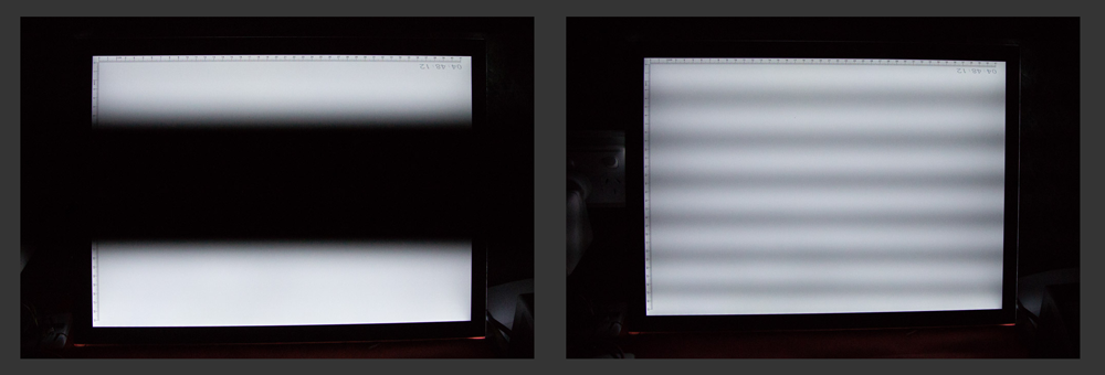
One of the potential problems with the LED based flats panel I described in a previous article is that if the exposure time used for flats is too short the resulting images can show banding - sometimes quite severely. The images below give a couple of examples.

Banding — Figure 1 - Illumination banding on an LED panel.

You may never encounter this problem but, in case you do, this article will explain why it happens and, more importantly, how you may be able to fix it.

The Cause

To put it simply, the cause is rolling shutter interference with the pulse-wave modulation of the panel but to understand this we need to look at how a camera's shutter actually works.

Consider first the case of an electronic shutter. You might reasonably assume that at the start of the exposure the shutter is turned on, it starts counting photons and at the end of the exposure the photon count values are read and the sensor is turned off. While this is largely true the actual situation is a little more complicated because it takes time to read a sensor and it is generally not possible to read the whole centre at once. Rather it is read line-by-line.

Now consider the following situation: we want to make a one second exposure on a 1000-line sensor that requires 0.01ms to read each line. If the sensor is turned on at time zero we can’t just turn it off again after one second because the data needs to be read out first and if the sensor is turned off the data will be lost. So after time 1s line 1 is read followed by lines 2, 3, 4 etc. and so on until the last line gets read until 100ms later. That means that line 1 will have been exposed for 1s but that each successive line will have received progressively longer exposures up to 1.01s for the 1000th line. Obviously this isn’t satisfactory. To ensure the exposure is even across the sensor the lines are also turned on progressively at the same rate as they are read. So, in this case, line 1 turns on at time zero but line 1000 doesn’t switch on until 10ms later. In this way every line gets the same 1s exposure.

Shutter animation 1 — Figure 2 - Typical DSLR shutter operation.

The situation is similar with a mechanical shutter where some kind of curtain arrangement is used to reveal and cover the sensor. To ensure even exposure a DSLR camera generally uses a focal plane shutter that consists of two separate curtains. At time zero the first curtain moves downwards to expose the sensor to light and at the end of the exposure a second curtain drops down over the sensor to block any further life before the sense is read. In this way each part of the sensor receives the same length of exposure. This two-curtain approach is shown in the animation in figure 2.

Hi Shutter Speeds

Now consider the sensor described above but where the exposure time is only 1/500th of a second (2ms). At time zero the first line switches on followed by subsequent lines each 0.01ms apart. After 2ms the exposure is complete and line 1 is read. However by that time only the first 200 lines have been switched on and so the reads are starting well before the whole sensor has begun to be exposed. The final line is not turned on until time 10ms and then finally read out 2ms later. Thus this 2ms exposure actually happens over a total period of 12ms.

Shutter animation 2 — Figure 3 - When the exposure time is shorter than the curtains' travel time.

The equivalent situation can occur with the mechanical shutter when the exposure time is shorter than the time it takes for the first curtain to fully open. In that case the second curtain starts to close before the first is completely open resulting in the shutter becoming a narrow slit which moves down over the sensor as shown in figure 3.

Imaging the LED Panel

Shutter animaton 3. — Figure 4 - A light source flashing too slowly for the exposure time.

Now let’s consider what happens when the flats panel is imaged. Recall that the panel has variable light intensity, which is achieved using pulse-wave modulation. While the LEDs always look evenly illuminated they are actually flickering on and off too rapidly for our eyes to detect - but not necessarily too fast for the camera to pick up. Returning return to our example of the 2ms exposure that takes 12ms to complete, if the LEDs are modulated at 250Hz they cycle on and off every 4ms. This means that they will have switched on and off three times during the exposure and, since only part of the sensor is being exposed at any given time, the travelling slit will not be consistently illuminated. The resulting image will show bands of light and dark as seen in figure 1 above. This process is demonstrated in the animation of figure 4.

Whether or not you see this phenomenon in your own flats will depend upon the combination of exposure time, PWM frequency and shutter raster speed for your particular setup, but it can happen. The images on the left of Figure one was taken with a Canon 5D Mark III DSLR using the panel as described in the previous article, that is, the default behaviour of Arduino PWM on pin 11.

The Solution

The panel appears evenly illuminated to our eyes because the pulsing is too fast for them to detect. Clearly, under certain circumstances, that pulsing is not fast enough to fool a camera and so the solution is to get the panel to modulate at a higher frequency.

To understand how to do that we first have to look at how that frequency comes about. Without going into details about how the pins are pulsed it is sufficient to know that each pair of PWM pins on an Arduino is controlled by an internal timer and that the basic operation is as follows.

The timer has two eight-bit registers, one is a counter and the other is a comparison register. The counter starts out at zero and the Arduino pin is switched on. At every tick of the clock one is added to the counter and it’s value is compared to the value in the comparison register and when the counter reaches that value the output pin is set to low. It remains low as the count continues until eventually the register overflows from 255 back to zero and the pin is turned back on. This is an oversimplification and each of the PWM have subtle differences but the principle is valid so one complete PWM cycle occurs in the time it takes for the counter to count to 256 (256 clock cycles) and the width of the pulses is controlled by setting the number in the comparison register, which is what the analogWrite command does. So the frequency of the PWM will be equal to the frequency of the clock divided by 256.

By default, on an Arduino with a 328 chip, the frequency or the relevant timer is 125kHz and so produces a PWM frequency of 125,000/256 ~ 488Hz. It would be possible to get a higher frequency by reducing the limit of the count. For example, if each cycle ended when the counter reached 64 then the frequency would be quadrupled to nearly 2kHz but this has the disadvantage that it reduces the resolution. The panel would then have only 64 distinct lighting levels rather than the 256 it has in normal operation. A better way is to increase the frequency of the clock that is driving it.

The timer’s clock is derived from the oscillator that runs the processor and that generally runs at 16MHz. However, that signal is passed through a divider that prescales it down. For pins 3 and 11 that prescale factor is 128 and hence the 16MHz frequency ends up down at 125kHz. The Arduino language does not provide a direct way to change those values but they are stored in registers within the processor chip and can be accessed with some more obscure code.

It turns out that the prescaler for these two pins is determined by the lower three bits of a register known as TCC2RB. Any value between 1 and 7 in these 3 bits is valid and will set a corresponding prescale value as shown in Table 1. In fact, it is possible to push the frequency even further by putting the timer into FastPWM mode by manipulating some bits in yet another register, TCCR2A. This halves each of the prescale values and hence doubles the PWM frequency.

Table 1 - Prescale PWM values and frequencies for pins 3 & 11.
Bits	Hex	Prescale p	Freq. f	Fast p	Fast f
001	1	2	32.25 kHz	1	62.5 kHz
010	2	16	3.91 kHz	8	7.81 kHz
011	3	64	977 Hz	32	1.95 kHz
100	4	128	488 Hz	64	977 Hz
101	5	256	244 Hz	128	488 Hz
110	6	512	122 Hz	256	244 Hz
111	7	2048	30.5 Hz	1024	61.0 Hz

Changing the PWM Frequency

So changing the frequency is just a matter of changing the appropriate three bits in the TCC2RB register which can be achieved by setting or resetting the bits as desired as shown below.

TCCR2B = TCCR2B & 0xf8 | 0x03;

This sets the bits to a value of 3 (011) and hence bumps the frequency up to 977Hz.

Similarly,

TCCR2B = TCCR2B & 0xf8 | 0x01;

would lift the frequency right up to 32.25kHz.

How how you will need to go depends upon circumstances but to switch into fast mode and list the frequency to 62.5kHz use the code,

TCCR2A = _BV(COM2A1) | _BV(COM2B1) | _BV(WGM21) | _BV(WGM20);
TCCR2B = 0x01;

Below is a modified version of the Arduino code which involves three modifications from the original.

A new method has been added to the Panel class to allow setting of the prescaler bits and hence setting the frequency.
The unit now runs in Fast PWM mode so the frequency can be set as high as 62.5kHz - which is the default start-up frequency.
A new command/response has been added so that the frequency can be changed via serial communication.

A new version of the PC test programme has also been created (available below) which adds the ability to choose PWM frequency.

If you are using the SGP compatible version of the Arduino software mentioned in the previous article then the PWM frequency can be modified by inserting one of the code snippets given above in the Setup function in between these two lines,

pinMode(ledPin, OUTPUT);
analogWrite(ledPin, 0);

Results

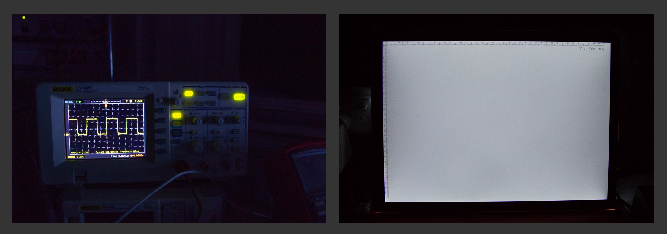
The image on the left of Figure 1 was taken with a Canon 5D Mark III with a shutter speed of 1/8000th of a second with the panel at its default frequency of 477Hz. While this is a very fast shutter speed the banding remains apparent right down to around 1/1000th of a second. The image on the right is the same camera and exposure but with the panel modulating at 3.9 kHz, which is clearly still not enough. Figure 5 below was taken with the panel operating at 62.5kHz and the banding has gone.

The frequency required to eliminate banding in your images will require some experimentation but it will hopefully be no more than the 62.5kHz demonstrated here.